Problem
In this exercise scenario, the refuge managers are in need of land cover data for management purposes of Black Water National Wildlife Refuge. The management plan calls for classification of the property based on an aerial photograph of the refuge and using image classification methodology.
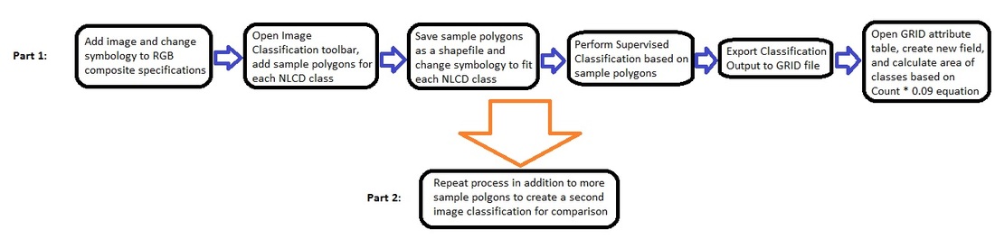
Analysis Procedures
This procedure used the same methodology of image classification for both Part 1 & 2. I began by adding the aerial .tif image and changing the symbology to RGB composite to the following values: Red Band 4, Green Band 3, and Blue Band 2. I then opened the Image Classification toolbar in my display and drew 2 polygon shapes around each area that represented NLCD classifications. Therefore I ended up with 2 polygons each for Water, Developed land, Barren Land, Cultivated land, Wetlands, and Forest. I then saved the sample polygons within the sample table to a shape file and added the shape file to my map. There I changed the symbology within the properties dialog box to display the appropriate classes and the NLCD colors associated with them. This was the symbology that I used throughout the rest of my procedure. From there, I chose the Interactive Supervised Classification option form the Image Classification toolbar and produced the .tif classification output which assigned the classes to the rest of the image based on the 12 sample polygons. Next, I found the new Classification 1 image output in the table of contents, and exported the data to a GRID raster file. From this point, I was able to open the attribute table of the GRID file and create a new field named Area. I used the Field calculator option to calculate the area based on the expression “Area = [COUNT] * 0.09”. After saving this first image classification, I then added more sample polygons to the original in order to improve the imagery. I added at least 3 more polygons to each class and exported the table to a shape file. I then used the same procedure as before to create a Supervised Classification of the image based on the addition of the new sample polygons. From there, I exported the .tif file to a GRID raster file and calculated the area using the same methods as the first classification.
Model:
Results
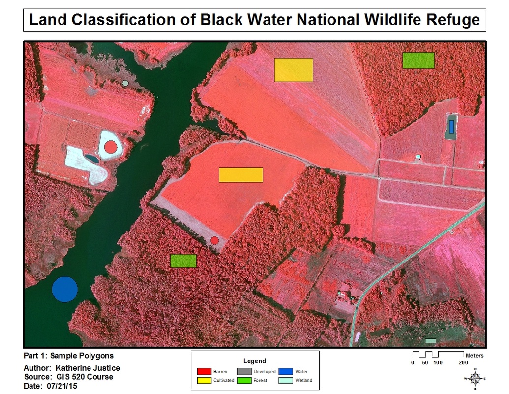
Part 1: Sample Polygons used for image classification of the Black Water National Wildlife Refuge. Only 2 polygons per class.
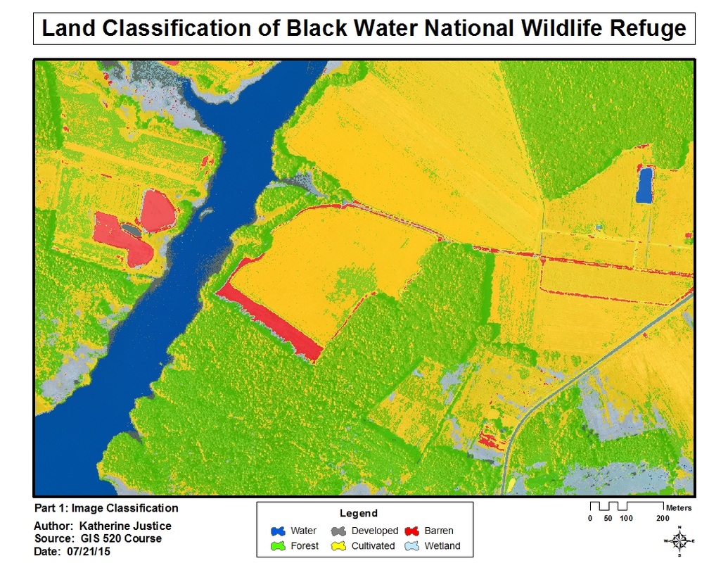
Part 1: Resulting image classification based on the Part 1 sample polygons. Noticeably incorrect patches of classification found in water, barren, and some forested areas.
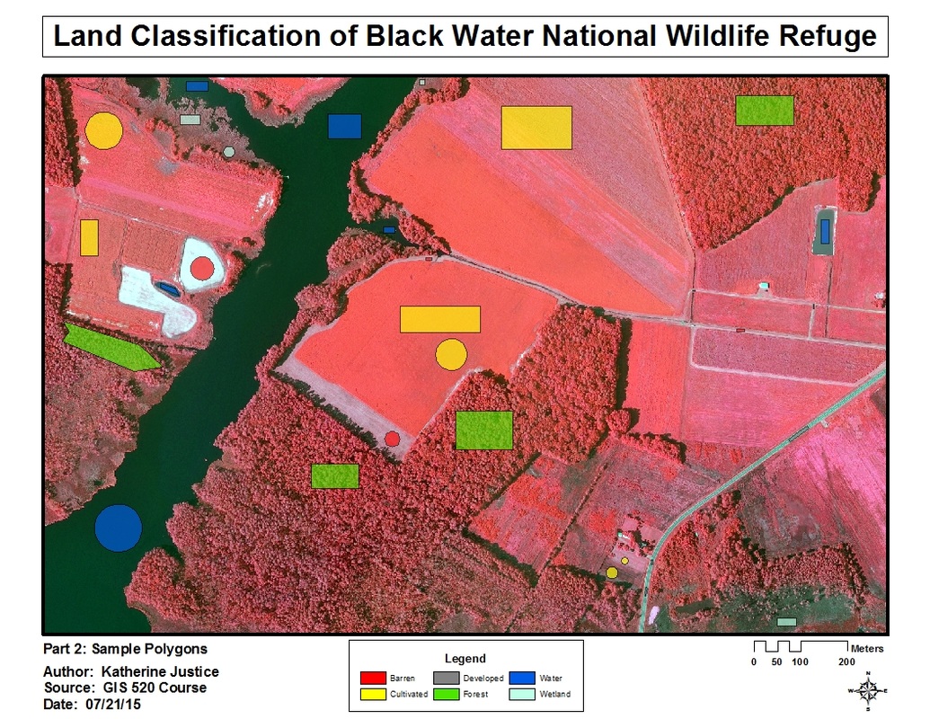
Part 2: Sample Polygons used for second image classification of the Black Water National Wildlife Refuge. Noticeably high number of polygons used for increased sample area.
Part 2:: Second resulting image classification based on the Part 2 sample polygons for comparison. Some areas have shown improvement, such as the classification of water and developed areas.

Appliction & Reflection
Although it took me some time to fully understand how to use the image classification toolbar, I believe that this skill will be a huge time saver for future projects. This tool saves the user time in that you only have to hand draw a few polygons to completely cover an entire land cover data image.I would note using smaller areas for each polygon in the future to ensure contiguous sampling for more accurate classification. Professionally, I would use this method for land management purposes. However, I could see this application being used further for development and transportation purposes as well. This would give an organization an ideal prospect of what land is workable and what is not. One example of this use would be if the Department of Transportation were looking to place a new bypass through undeveloped land. They wouldn’t want to place a road through a wetland due to environmental and longevity reasons, so they could use this to locate land in upland areas and areas closer to commercial use.
